Associated publication
Feel free to use this work, however, if you are using it for your research please cite the following paper :
Semi-automatic extraction of functional dynamic networks describing patient’s epileptic seizures [pdf] [frontiers]
Gaëtan Frusque, Pierre Borgnat, Paulo Gonçalves, Julien Jung,
Frontiers in Neurology, 09-2020
Overview of the codes provided
BTNDmain.m: Main file, divided in two parts. First, an example using functional connectivity (FC) data from 3 seizures of a patient with:
-
DataFC.mat: The FC matrix of the 3 seizures (DataFC{i} is the FC matrix from the seizure i).
-
NameCoordinate.mat: Name of the electrodes indicating their positions in the brain (used to visualise the result).
Then, a second part explains how to apply the code with your dataset (see also section “Description of the method”).
FC_dynamic.m: Compute a time-varying network for each seizure with an FC measure. The arguments are Signal the list of seizure recordings; method the FC measures used (Pearson correlation, Phase Locking Value or Amplitude Envelope Correlation); Freq the sampling frequency; TimeSegment the size of the temporal segments (in s) used to compute an FC graph; Step a graph is computed at every ‘Step’ second.
BTND.m: Decompose the time-varying network using the criteria (3) from the article. The arguments are X the time-varying network represented as a list of FC matrices; K number of subgraph wanted; [lambda,gamma,eta] the three parameters of the BTND; init number of different initialisations.
The output of the BTND are F containing the K subgraphs (in the columns of the matrix); V containing the activation profile of each subgraph specific to each seizure (V{i} activation profiles related to the seizure i); cost cost function values at each iteration of the algorithm.
The BTND is solved by alternating two steps :
-
BTND_LassoRegression.m: Compute the matrix F knowing matrices V{1}, V{2}, …, V{N} by performing a lasso regression.
-
BTND_FusedRegression.m: Compute matrices V{1}, V{2}, …, V{N} knowing F by performing a regression under Fused lasso constraints. The projection on the Fused lasso constraint is done using algorithm TV_Condat_v2.m from the website of Laurent Condat.
DISPLAY_graphcreate.m: Tool to visualise the matrix F as K circular graphs.
Desciption of the method
We describe here our novel semi-automatic method to characterise the dynamic epileptogenic network quantitatively and across time using SEEG signals.
Overview
For each patient, the dataset is composed of several SEEG recordings for different seizures. Seizures can have different durations. The proposed strategy can be summarised in four steps:
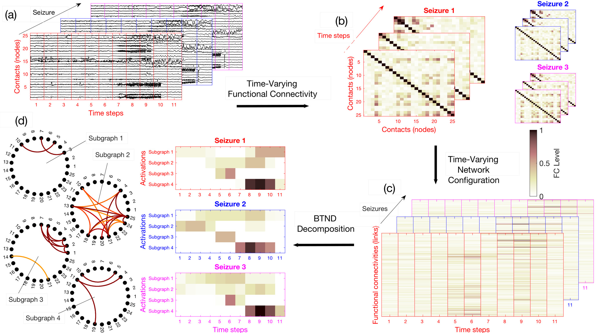
(a) We chop each recording into short segments,
(b) For each segment, we estimate via FC measures, the connectivity for each pair of electrode contacts.
(c) We rearrange the FC measures into a list of matrices representing the time evolution of FC for each seizure of a patient.
(d) The list of matrices representing the multi-seizures brain-wide time-varying network is decomposed into FC subgraphs characteristic of one patient but common to all his seizures, along with their activation profile specific to each seizure.
The main steps of the method are illustrated in the figure 1 of the paper:

We provide now the code to perform all the steps presented in this figure.
1 - Get the data
In order to use the BTND pipeline, the dataset has to be arranged as a list of recording (as illustrated in figure 1.(a) of the paper).
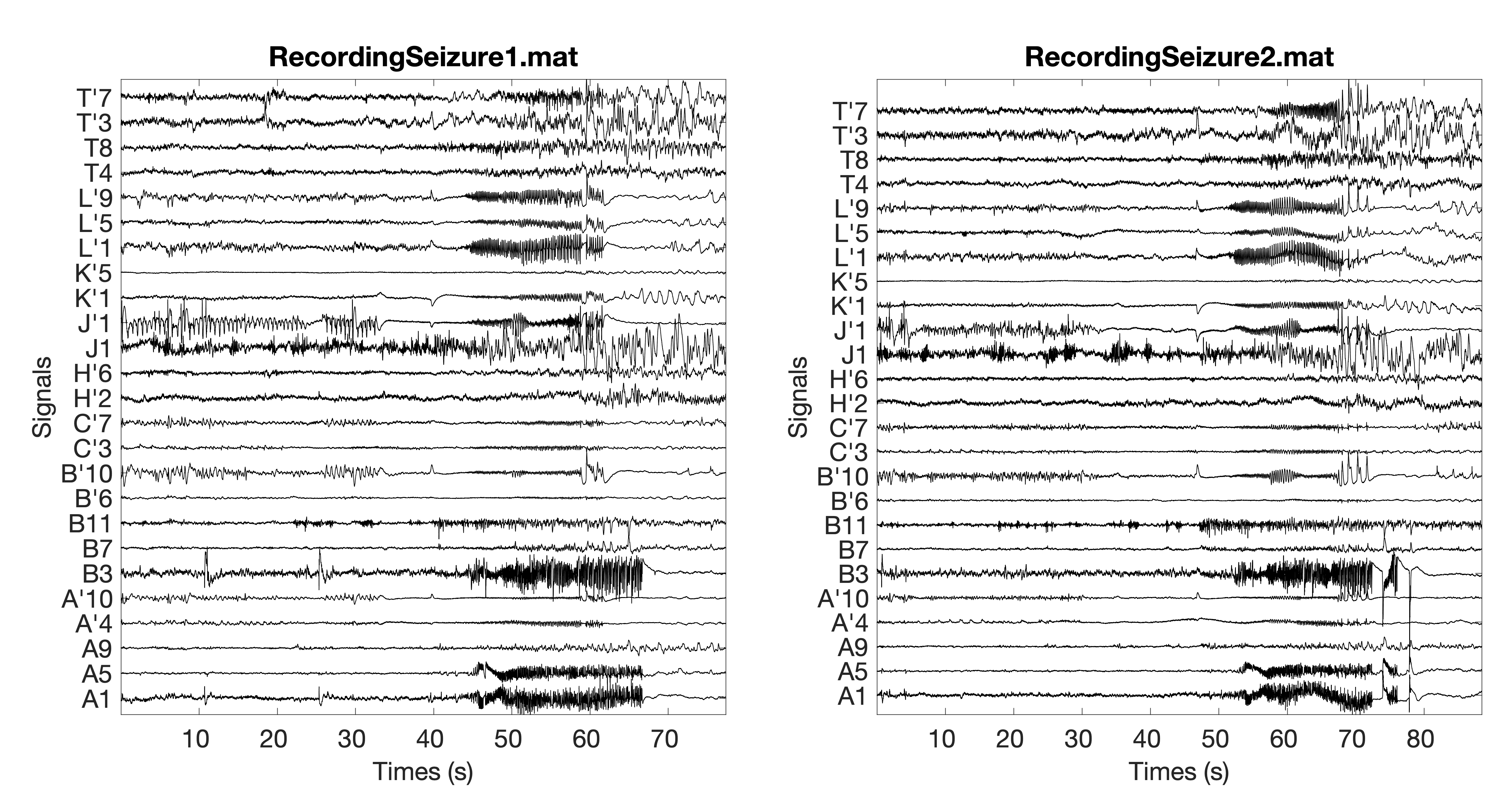
Considering, as an example, two recordings named “RecordingSeizure1.mat” and “RecordingSeizure2.mat” illustrated here:
 Then a variable Signal have to be created with :
- Signal{1} = RecordingSeizure1 (matrix channel x time1)
- Signal{2} = RecordingSeizure2 (matrix channel x time2)
Notice the recordings must be cleaned from artefact and filtered in a bandwidth of interest before. Also, The duration can differ from one recording to another. However, the number of channels must stay the same.
2 - Time-varying network inference
Now we compute a time-varying network for each seizure in the variable Signal with an FC measure. The multi-seizures time-varying network is represented as a list of FC matrices noted by the variable X.
The function FC_dynamic.m directly entails the transition from the step figure 1.(a) to 1.(c) of the paper. It performs at the same time the time-varying functional connectivity computation and the reconfiguration as a list of FC matrices. We have :
- X = FC_dynamic(Signal, method, Freq, TimeSegment, Step);
Three measures of FC are already implemented to construct the networks. Use as argument method = ‘PLV’ for the Phase Locking Value (FC measure used in the paper), method = ‘COR’ for the Pearson correlation and method = ‘AEC’ for the amplitude envelope correlation.
Argument Freq (Hz) corresponds to the sampling frequency of the recordings. Arguments TimeSegment (s) and Step (s) are the main parameters to infer the dynamical network: A graph is computed at every Step second using a rectangular window of TimeSegment seconds.
3 - BTND
We can now decompose the time-varying network represented by the variable X in K subgraphs with their corresponding activation profiles for each seizure. Notice X is a list of matrix, with X{i} the time-varying network of the seizure i.
Note : X can be computed using other function than “FC_dynamic” (for example using brainstorm functions). Then, X{i} have to be a matrix of dimension “Functional connectity x time(i)” (the time can differ from one network to another bust the number of Functional connectity must stay the same). In this case, be carefull using the “DISPLAY_graphcreate” function, the ordering of the functional connectivities can become different inducing mismatched activation on the sub-graphs.
The function BTND.m entails the transition from the step figure 1.(c) to 1.(d) of the paper. Decomposing the time-varying network using the criteria (3) from the article. We have:
- [F, V] = BTND(X,K,[lambda,gamma,eta],init)
with F in a matrix of dimension “links x K”. It is a mathematical representation the K subgraphs (whose information is contained in the columns of the matrix). V contains the activation profile of each subgraph specific to each seizure (V{i} activation profiles related to the seizure i, with dimension “time(i) x K”).
The differents argments are:
-
K (scalar) the number of subgraphs wanted.
- lambda, gamma and eta the \(\lambda\), \(\gamma\) and \(\eta\) parameters from the equation (3) of the paper. We remind that lambda and gamma are limit the number of non-zeros elements in respectively the subgraph’s links and the activation profiles. \(\gamma\) is the temporal smoothing of the activation profiles. As presented in the supp material, considering \({\rm \mathbf{X}} \in \mathbb{R}^{L \times T(s)}\), then \(\gamma_s = T(1)/T(S) \gamma\) and \(\eta_s = T(1)/T(S) \eta\). The parameters \(\gamma_s\) and \(\eta_s\) vary in function of the duration of the seizure.
- init: because the criteria (3) is non convex, different initialisations can lead to different solutions. we compute for init different initialisations a locales minimum of the criteria (3) and retain the best result
Recommendations for the parameters selection: We recommend first to merge the sparsity parameters \(\lambda\)=\(\gamma\) (same value). There is now two parameters to select: \(\lambda\) and \(\eta\). The user can play with these two parameters, we propose in BTNDmain.m a configuration that work well most of the time in our dataset \(\lambda\)=0.4 and \(\eta\)=0.2. In the paper, we fixed \(\eta\)=0.2 and selected the \(\lambda\)=0.4 according to a rule discribed in the Supplementary Material. We quickly describe the rule: considering the following score \(a_{\lambda} = \sum_{s=1}^{S} { \mid \mid \mathbf{X}\{s\} - \mathbf{F} \mathbf{V}^t\{s\} \mid \mid^2_F}\). We consider the value of this score when \(\lambda\)=0 and \(\lambda=\infty\) (corresponding to \(a_{\infty} = \sum_{s=1}^{S} { \mid \mid \mathbf{X}\{s\} \mid \mid^2_F}\).). The we are looking for a compromise between no regularisation and a too strong regularisation by looking for the value of \(\lambda\) such as \({a_\lambda \approx 0.8(a_{\infty} - a_{0}) + a_{0}}\). Thanks to this value of \(\lambda\), we only selected subgraphs that contain few FC to characterise a delimited temporal event of the seizures for each patient.
An example of settings that often worked fine on our dataset :
-
\(\lambda\) = \(\gamma\) = 0.4
-
\(\eta\) = 0.2
-
K=5
-
init=2 (then init=20 if you are satisfied with results obtained thanks to the settings above).
4 - Visualisation
We propose at the end of the BTNDmain.m tools to visualise the F matrice as K circular graphs, and to represent the V{s} activation profiles. These representations are similar to the figure 2-5 of the paper.